A decision tree is a popular method of creating and visualizing predictive models and algorithms. You may be most familiar with decision trees in the context of flow charts. Starting at the top, you answer questions, which lead you to subsequent questions. Eventually, you arrive at the terminus which provides your answer. (If you are unfamiliar with flow charts, this humorous image illustrates the concept.)
Decision trees tend to be the method of choice for predictive modeling because they are relatively easy to understand and are also very effective. The basic goal of a decision tree is to split a population of data into smaller segments. There are two stages to prediction. The first stage is training the model—this is where the tree is built, tested, and optimized by using an existing collection of data. In the second stage, you actually use the model to predict an unknown outcome. We’ll explain this more in-depth later in this post.
A very thorough article that describes what a decision tree is and what they can be used for. They are my favorite first step in doing most kinds of data modeling. Even though they may not be the most sophisticated algorithm, they provide very good insight into the data. The output of a decision tree is easily readable up the organization, so communication of findings is much easier than more sophisticated, blackbox modeling techniques such as neural nets.
When it comes to actually building a decision tree, we start at the root, which includes the total population of atoms. As we move down the tree, the goal is to split the total population into smaller and smaller subsets of atoms at each node; hence the popular description, “divide and conquer.” Each subset should be as distinct as possible in terms of the target indicator. For example, if you are looking at high- vs. low-risk customers, you would want to split each node into two subsets; one with mostly high-risk customers, and the other with mostly low-risk customers.
This goal is achieved by iterating through each indicator as it relates to the target indicator, and then choosing the indicator that best splits the data into two smaller nodes. As the computer iterates through each indicator-target pair, it calculates the Gini Coefficient, which is a mathematical calculation that is used to determine the best indicator to use for that particular split. The Gini Coefficient is a score between 0 and 1, with 1 being the best split, and 0 being the worst. The computer chooses the indicator that has the highest Gini Coefficient to split the node, and then moves on to the next node and repeats the process.
This gets a little into the weeds, but effectively the computer decides which variable is the best indicator at predicting the target. Once it does that, it continually iterates through each branch of the data and picks out the best variable for the next group. It does this until there is not a good split for the data and then it ends the branch.
This is why I love decision trees. Each subset gets tighter and tighter as it goes down a branch. This is where "art" comes into the science. Even though a tree may not be good at predicting the future, it provides great insight in the data for testing.

Decision Trees can be anywhere from really simple.
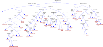
To much more complex and everywhere in between and beyond.
For example, the target variable could be high-worth customers. The branch may break off on gender of female, region of South and age between 35 - 55. This group is said to be likely high-worth. A good testing hypothesis is to find all the females aged 35-55 that live in the South who are not high-worth and see if they may have a higher propensity to spend with you than they currently are. Now this is a simplistic example and this general of a group will probably not show up on a tree, but you get the idea.